Lecture 4 - Follow Frequency Response

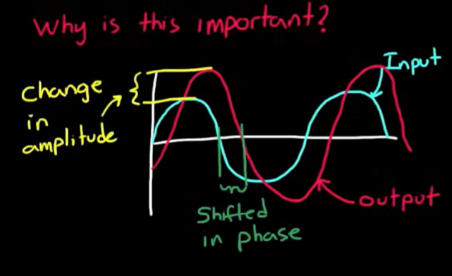
Why sine in → sine out?

• Linear time invariant (LTI) systems can only do a few things on the input (gain, derivative, integration, addition/subtraction)
• These operations only change the magnitude and phase of the input sine signal without changing frequency
• Thus, the gain and phase shift provided by the LTI change by changing the frequency of the input (i.e. gain and phase shift of the transfer function are a function of the input frequency)
• Sinusoidal signals are the only repeating inputs whose waveform (shape of the signal which is governed by frequency) is not changed when fed into an LTI system

Why those crazy plots?

• Time domain is only practical to visualize the output of a single input frequency, otherwise the plot will be overflowed by sine curves overlapping each other

  

• Since the frequency is what only affects of an LTI is only influenced by frequency, we want to visualize the gain and phase shift over a whole spectrum of input frequencies

• One of those crazy plots that help us do so is the Bode Plot

The Bode plot

Why dB and log scale?

• In bode plot, gain is not plotted directly
  • we first find the amplitude ratio between the input and output, square that to get power ratio, take the log base 10 of the result, multiply that by 10 and get $20{\log }_{10}(\text{out/in})$
  • Note: that out/in is just the gain ($k$) of the transfer function
• But why all of that?
  • When working with telephone lines, they found that $10{\log }_{10}(\text{power loss})$ is the smallest attenuation detectable by the human ear due to power loss. They called that “Decibel”
  • $\text{power}\propto$ ${\text{amplitude}}^2$, so $10{\log }_{10}(\text{power})\propto 10{\log }_{10}({\text{amplitude}}^2)$
  • From properties of logarithm, we get $20{\log }_{10}(\text{amplitude})$. We want to use gain ($k=$(ratio between output and input amplitudes) instead of the amplitude of the output to see how the amplitude changed
  • So we end up at $20{\log }_{10}(\text{out/in})=20{\log }_{10}(k)$
  • But does this have to do with telephone lines anyways?? Read more and you will find out!
• Why log scale for frequency?
  • We get to plot the output for a wide spectrum of frequencies

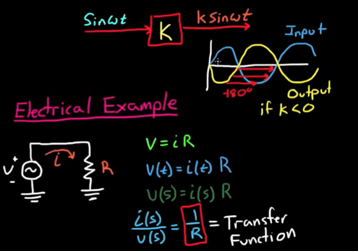
How do we compute gain and phase shift?

We can use trig! We feed a general sinusoidal input of amplitude $A$, frequency $\omega$, and phase $\varphi$ to the system, find the output, then compute the gain (amplitude of output / amplitude of input; can be converted to $dB$) and phase shift (phase of output - phase of input)

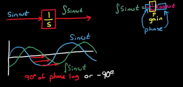We can use the transfer function itself

• How can the transfer function help with this? We just have a bunch of $s$ terms?
• Actually $s=\sigma +j\omega$ (that is by definition)
• The $\sigma$ term is responsible for the transient response (output of the system), but we are interested in the steady state response (which is governed by $j\omega$)
• So, for a sinusoidal input, $s$ becomes $j\omega$ at stead state

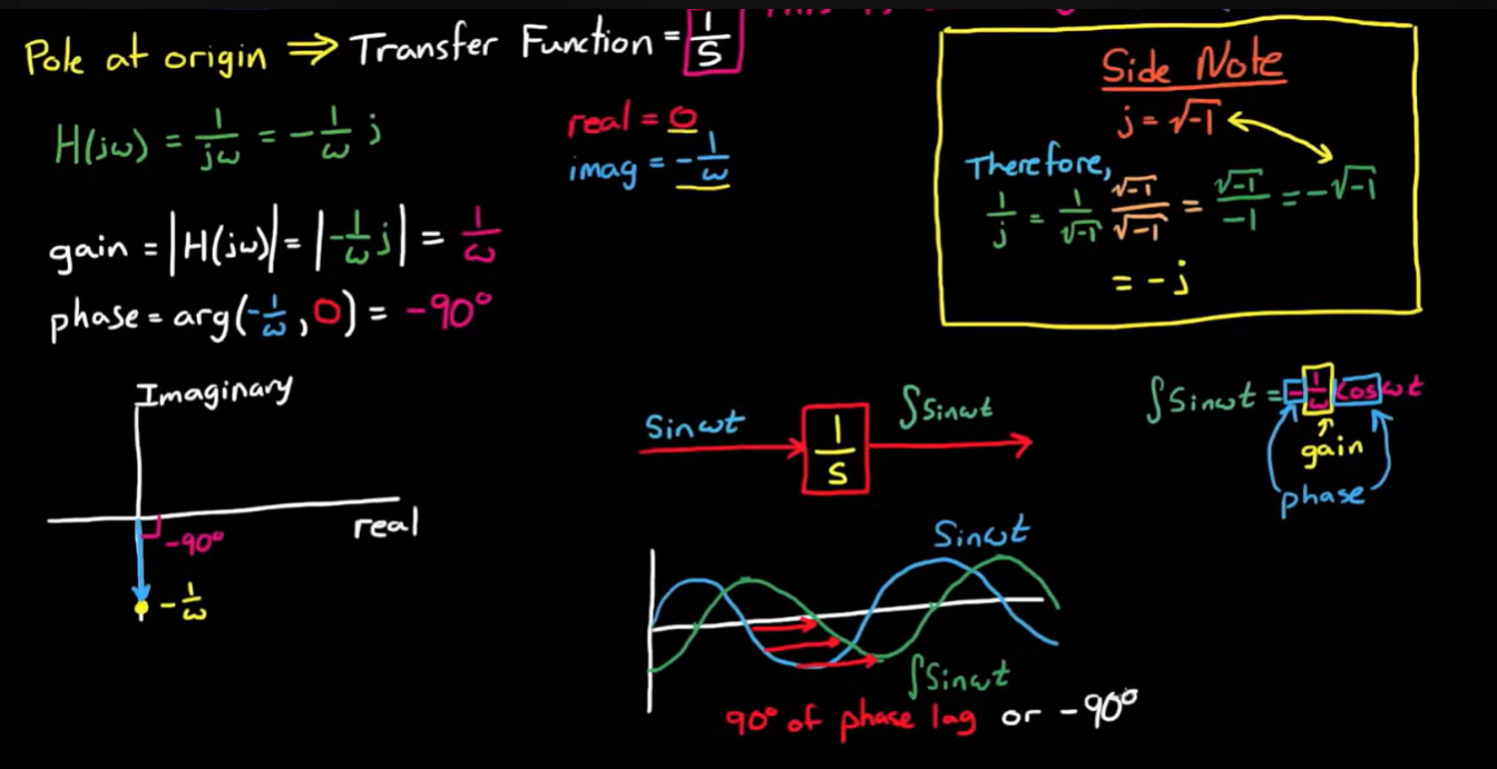
We can calculate steady state gain and phase shift by

• Finding the transfer function
• setting $s=j\omega$
• Manipulating the transfer function so that it has a real component and an imaginary component
• Plotting the transfer function on the real and imaginary axis
• Calculating gain and phase from this plot
  • Gain = magnitude of the line from the origin to the point
  • Phase = angle of the line with the x axis
• Note: we can calculate gain and phase without having to manipulate the transfer function to have a real component and an imaginary component:
  • Gain = magnitude of numerator / magnitude of denominator
    • In general, multiplied terms = multiplied amplitudes and divided terms = divided amplitudes
  • Phase = phase of numerator - phase of denominator
    • In general, multiplied terms = added phases and divided terms = subtracted phases

Let’s apply this on the gain transfer function:

Is there a faster way? Yes!

You can plot the gain and phase directly from the transfer function without needing to manipulate it!

How to compute the output directly from the transfer function?

Why bother about manual sketching when we have MATLAB?

• Just by looking at the transfer function, you can predict the frequency response of the system
• Just by looking at the frequency response of a system, you can predict the transfer function of the system How do we sketch from the transfer function directly? We use poles and zeros
• We will use the slow method of manipulating the transfer function on the most common transfer functions:
  • No poles or zeros: $k$ (gain)
  • At the origin
    • Pole at origin: $\frac{1}{s}$ (integrator)
    • Zero at origin: $s$ (differentiator)
  • Real
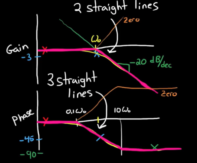
    • Real pole: $\frac{1}{\tau s+1}$
    • Real zero: $\tau s+1$
  • Complex
    • Complex pole: $\frac{{\omega }_o^2}{s^2+2\zeta {\omega }_{o}s+{\omega }_o^2}$
    • Complex zero: $\frac{s^2+2\zeta {\omega }_{o}s+{\omega }_o^2}{{\omega }_o^2}$
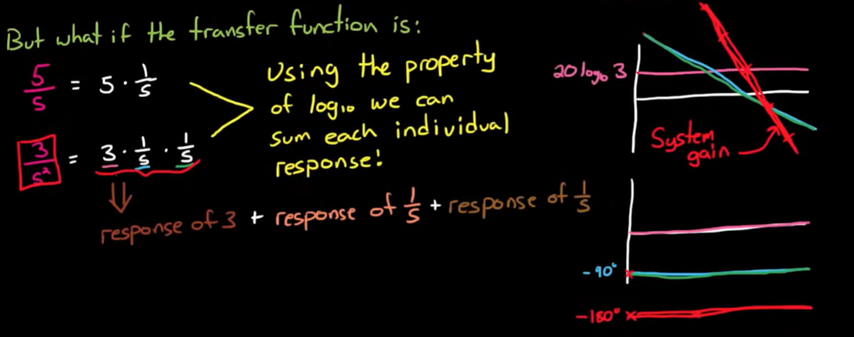
• These our building blocks for any other complex transfer function (any other complex transfer function is just the multiplication of these simple transfer functions together)
• If we know how to plot these, then plotting any other complex transfer function is just a matter of adding the plots of these building blocks together

This is an advantage of using $dB$ gains! (in the log world, multiplication becomes addition and division becomes subtraction)

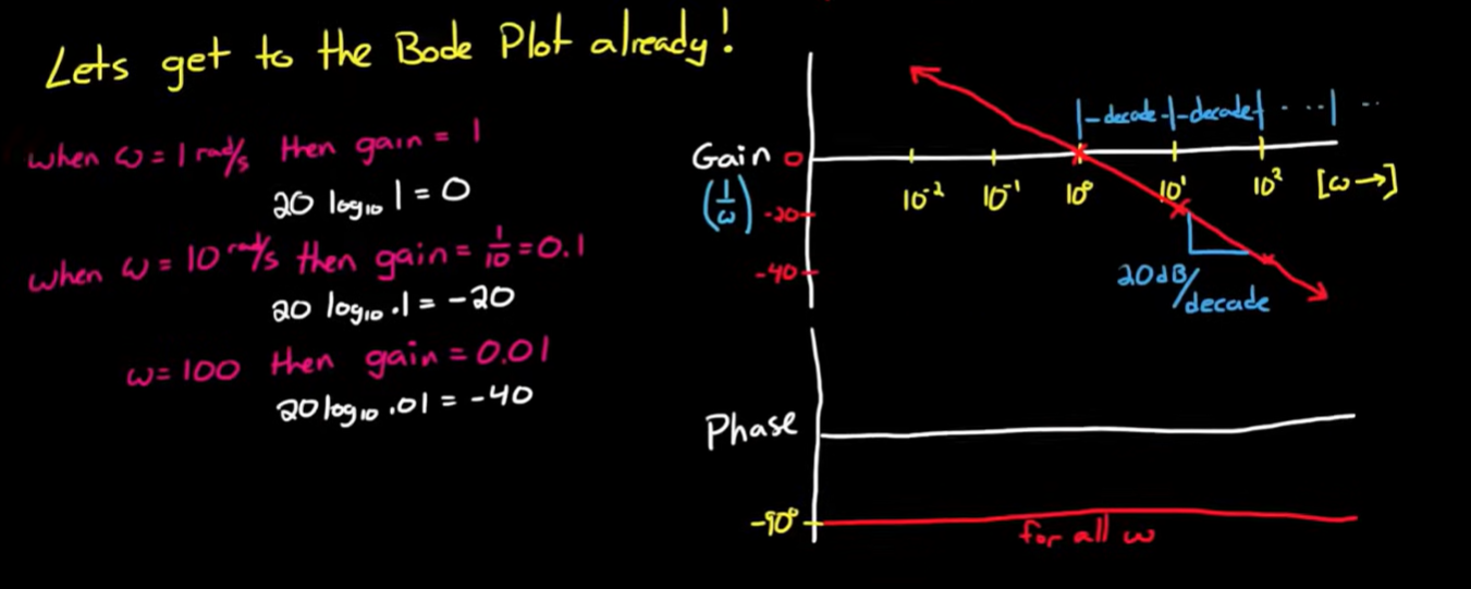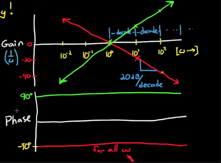
We already know the gain $k$. Let’s consider pole at origin $\frac{1}{s}$: How do we extend this? Multiplication becomes addition in the log world Division becomes subtraction in the log world Zero at origin: $s$

$$s=\frac{1}{1/s}$$

in log world: response of $s$ $=$ response of $1$ - response of $1/s$ Lets consider real poles $\frac{1}{\tau s+1}$ How to extend this for real zero $\tau s+1$? $\tau s+1=\frac{1}{\left(\frac{1}{\tau s+1}\right)}$ Division becomes subtraction in the log world

response of zero = - response of pole

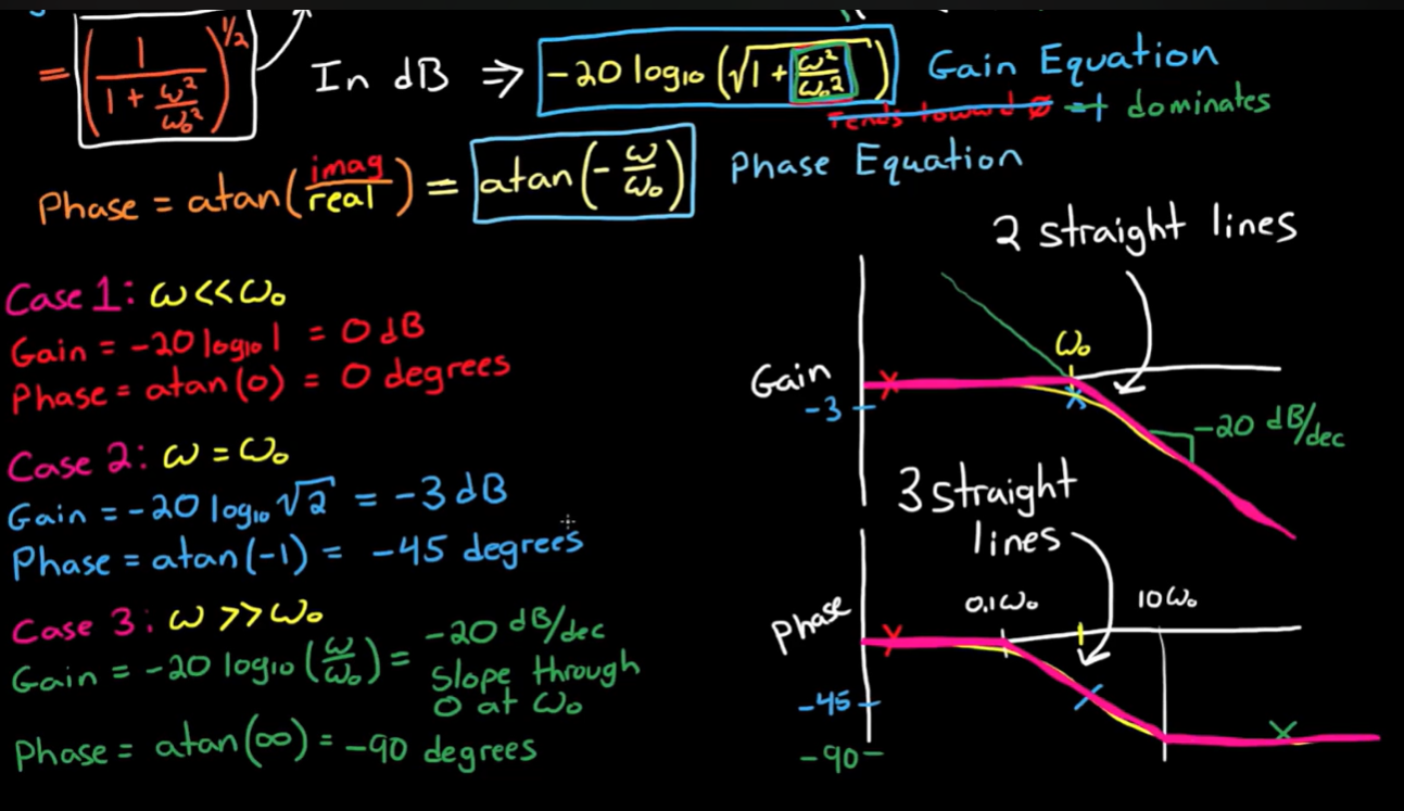
Let’s consider complex poles $\frac{{\omega }_o^2}{s^2+2\zeta {\omega }_{o}s+{\omega }_o^2}$

• Bode Plots by Hand: Complex Poles or Zeros
• CORRECTION: Bode Plots by Hand: Complex Poles or Zeros

Summarizing frequency responses

In general, zero = - pole

---

General Remarks

• Plotting an arbitrary transfer function = superposition of simpler transfer functions
• Polar method = start from $|G(j\omega )|$ and $\varphi$ as $\omega \to 0$ then approach $|G(j\omega )|$ and $\varphi$ as $\omega \to \infty$

Resources

• Lecture 3_ Frequency Response.pdf
• Control Systems Plots
• Map of Control Theory
• Classical Control Theory, Section 2: Those crazy plots!